Data analysis and results
Overview
Teaching: 20 min
Exercises: 0 minQuestions
What is the role of data wrangling?
What are good practices for keeping code in check?
How to use data visualisation for insight and communication?
Objectives
First learning objective. (FIXME)
To make informed decisions using data.
Data Wrangling and Cleaning
Data wrangling involves cleaning data so it can be easily read and analysed by machines. It can also involve integration, extraction, removing missing points, and anything that makes data useable and functional. Regardless of the methods, the code involved with data cleaning steps should be carefully documented so that the steps involved can be repeated from raw data to cleaned data.
When working with data sets,
ggplot(in R) ormatplotlib/seaborn(in Python) libraries provide attractive figures that can be produced very quickly. Visualising data should not not wait for the point of publication, and can be used to explore data from the start, and also illustrate methodology. This is particularly valuable in Jupyter Notebooks. Code to produce figures should be literate, functional, reuseable in the same way as data cleaning and analysis code. That way future visualisations can be easily updated or reused.
Data wrangling
Definition
Data wrangling—also called data cleaning, data remediation, or data munging—refers to a variety of processes designed to transform raw data into more readily used formats. The exact methods differ from project to project depending on the data you’re leveraging and the goal you’re trying to achieve.
Some examples of data wrangling include:
- Merging multiple data sources into a single dataset for analysis,
- Identifying gaps in data (for example, empty cells in a spreadsheet) and either filling or deleting them,
- Deleting data that’s either unnecessary or irrelevant to the project you’re working on,
- Identifying extreme outliers in data and either explaining the discrepancies or removing them so that analysis can take place.
Data wrangling can be a manual or automated process. In scenarios where datasets are exceptionally large, automated data cleaning becomes a necessity.
Data Wrangling steps
Each data project requires a unique approach to ensure its final dataset is reliable and accessible. That being said, several processes typically inform the approach. These are commonly referred to as data wrangling steps or activities.
Discovery
Discovery refers to the process of familiarizing yourself with data so you can conceptualize how you might use it. You can liken it to looking in your refrigerator before cooking a meal to see what ingredients you have at your disposal.
During discovery, you may identify trends or patterns in the data, along with obvious issues, such as missing or incomplete values that need to be addressed. This is an important step, as it will inform every activity that comes afterward.
Structuring
Raw data is typically unusable in its raw state because it’s either incomplete or misformatted for its intended application. Data structuring is the process of taking raw data and transforming it to be more readily leveraged. The form your data takes will depend on the analytical model you use to interpret it.
Cleaning
Data cleaning is the process of removing inherent errors in data that might distort your analysis or render it less valuable. Cleaning can come in different forms, including deleting empty cells or rows, removing outliers, and standardizing inputs. The goal of data cleaning is to ensure there are no errors (or as few as possible) that could influence your final analysis.
Enriching
Once you understand your existing data and have transformed it into a more usable state, you must determine whether you have all of the data necessary for the project at hand. If not, you may choose to enrich or augment your data by incorporating values from other datasets. For this reason, it’s important to understand what other data is available for use.
If you decide that enrichment is necessary, you need to repeat the steps above for any new data.
Validating
Data validation refers to the process of verifying that your data is both consistent and of a high enough quality. During validation, you may discover issues you need to resolve or conclude that your data is ready to be analyzed. Validation is typically achieved through various automated processes and requires programming.
Publishing
Once your data has been validated, you can publish it. This involves making it available to others within your organization for analysis. The format you use to share the information—such as a written report or electronic file—will depend on your data and the organization’s goals.
Importance of Data Wrangling
Any analyses you perform will ultimately be constrained by the data that informs you. If data is incomplete, unreliable, or faulty, then analyses will be too—diminishing the value of any insights gleaned.
Data wrangling seeks to remove that risk by ensuring data is in a reliable state before it’s analyzed and leveraged. This makes it a critical part of the analytical process.
It’s important to note that data wrangling can be time-consuming and taxing on resources, particularly when done manually. This is why many organizations institute policies and best practices that help employees streamline the data cleanup process—for example, requiring that data include certain information or be in a specific format before it’s uploaded to a database.
For this reason, it’s vital to understand the steps of the data wrangling process and the negative outcomes associated with incorrect or faulty data.
Code that cleans and processes data (processing code) provides the very beginning of the data analysis pipeline: starting with raw data and resulting in processed data.

Cleaning data means it can be easily read and analysed by machines and used in analysis pipelines. It can involve changing labels, subsetting, integration, extraction, removing missing points, and anything that makes data useable and functional. Regardless of the methods, the code involved in data cleaning steps should be carefully documented so that the steps involved can be repeated from raw data to clean data. When reviewing this type of code, consider whether the steps involved are readable and in the correct order.
Case study example:
A PhD student has recorded lab results in an Excel spreadsheet. She has a copy of the raw results, but for her analysis, she wants to remove some outliers. She manually deletes some rows and saves the data as .csv. There is no record of what she deleted or the rule she applied, and a manual check of the differences between her data and the original would be necessary.
Instead, another PhD student writes an R script that reads the raw data file, uses a filter where the method and parameters are saved, and saves the output as a CSV file. Her process for removing outliers is reproducible.
Within a computational project, these steps may accidentally become obscure and so specific effort is required to make sure no one is manually processing data in a way that can’t be repeated and that all the steps are recorded.
genomeProject/processing/data_cleaning.py

import pandas as `pd`

# Reads raw data from a directory.
df = pd.read_csv('genomeProject/data/220103_GenomicData.csv')

# Shows the first 5 rows of the data set.
df.head(5)

# Remove unwanted columns by name
df.drop(columns=['year','quasi_column_ID'],inplace=True)

# Rename a column name
df.rename(columns={"batch_3_4_7": "batch_347"})

# Shows the first 5 rows of the data set now with the columns renamed and some removed
df.head(5)

# Change the index of the data to an ID
df = df.set_index('ID')

# Save processed data set
df.to_csv(genomeProject/data/220103_GenomicData_processed)
Data exploration and insights
The first part of data analysis is exploration. It is usually helpful to look at the data directly, and this might involve:
- Printing rows of a dataset in a notebook/IDE
- Printing the summary statistics for each row of a column
- Producing a scatter plot or histogram for a column of data
Visualising processed data before any analysis is usually always helpful.
When working with data sets, ggplot (in R) or matplotlib/seaborn (in Python) libraries provide attractive figures that can be produced very quickly. Visualising data is useful for exploring data from the start, and also illustrates the methodology or the steps of analysis.
This is particularly valuable in Jupyter Notebooks. Code to produce figures should be literate, functional, and reusable in the same way as data cleaning and analysis code.
That way future visualisations can be easily updated or reused.
Unlike data visualisations for release/communicating results/publications, these figures may be more practical than aesthetic. It is perfectly acceptable to open 25 histograms at once when exploring data, even though in an eventual paper you would only show one. Data visualisation is a tool, and small functions or scripts can make sure exploring data is practical and easy to repeat.
The code to produce the following figure is below.
Libraries like matplotlib do a lot of the hard work for you, and there are countless tutorials for different kinds of visualisations.

plt.hexbin(x, y, gridsize=30, cmap='Blues')
cb = plt.colorbar(label='count in bin')
Data Analysis and Statistics
(Need to discuss this further, what is patronising?)
With readable, clean, processed data that you have explored using figures, the next stage of the data pipeline is analysis. There may be many variables that are related directly or indirectly to the objective. For that, we first need to study about all the variables whether it is nominal or ordinal. Preparing the data for analysis is done after understanding the data. While understanding we get to know about missing in the data, finding the independent and dependent variables, etc.
Depending on your computational project, this may involve elaborate and complex analyses, modelling, simulation, and even machine learning. However, even if this step is just running a single statistics test, keeping the code modular in clearly defined steps is key.
Here is an example of applying a Butterworth filter to some data in Python. The specifics don’t matter, you can consider this code pseudocode for any kind of analysis step.
genomeProject/analysis/01_butterworth_filter.py


import numpy as np
from scipy.signal import butter,filtfilt

# (A) Read processed data from file
df = pd.read_csv('genomeProject/data/220103_GenomicData_processed.csv')

# (B) Defining filter parameters
T = 5.0         # Sample Period
fs = 30.0       # sample rate, Hz
cutoff = 2      # desired cutoff frequency of the filter, Hz
nyq = 0.5 * fs  # Nyquist Frequency
order = 2       # quadratic
n = int(T * fs) # total number of samples

# (C) Define the Butterworth Filter Function
def butter_lowpass_filter(data, cutoff, fs, order):
    normal_cutoff = cutoff / nyq

    # Get the filter coefficients
    b, a = butter(order, normal_cutoff, btype='low', analog=False)
    filtered_data = filtfilt(b, a, data)

    return filtered_data

# (D) Apply Butterworth Filter Function to the data
filtered_data = butter_lowpass_filter(data, cutoff, fs, order)
(A) the processed data is read into the script. Next, (B) the fixed parameters are set and named with comments.
These fixed numbers are saved as variables with names. In (C) the filter itself is written as a Python Function, which means it can be called multiple times throughout the script.
Because the parameters are not written into the function directly (so it doesn’t say b, a = butter(2, 15,btype='low', analog=False) but instead uses variables) this code is reusable without having to paste and edit the numbers every time you apply a function.
You can also call this function in other scripts. It can make sense to produce a file with the functions inside that can be imported into different scripts in case other projects also have similar methods. This is known as a package or library. This means altering a function doesn’t mean searching across every file on every project and changing it dozens of times.
Case Study
A postdoc wrote a helpful series of functions for data analysis with neurophysiology recordings. The postdoc wrote them as reuseable, and so two PhD students copied and pasted these blocks of code into their code and used it to analyse the data for their projects.
The postdoc later discovers a better way of writing the functions. One PhD student also wants to change the method and so has to search through his files to replace the code. The other PhD student wants the old method in some files and the new method in others, and so does not change all of them. It is therefore complex to follow the differences in the methods across the projects, and this is very open to errors in typos.
Instead, the postdoc could have saved his functions in the lab’s private repo which becomes the master copy and students pull from this. With the functions saved in a library, the PhD students can import them into their scripts. Now when the postdoc changes the functions and saves them to the repo, PhD students can choose to update their version of the functions. The students should document which version they have used.
The output of the analysis code may be statistics results that are reported in a paper, and therefore the steps required to reproduce them are critically important.
Figures for Communicating Results
With the analysis complete, data visualisation is usually used to communicate results. The code used to produce figures is the next step in the data pipeline.
For publications or posters, well-constructed figures improve science communication and help improve the impact of your research. Being able to produce multipanel figures with annotations and different colour schemes is complex but one of the advantages of learning a data science language.
It is therefore worth taking the time for researchers to learn the technical skills in R, Python, or another language to produce visualisations. Producing figures in Excel is limiting and often frustrating, particularly as there are only limited options in layout and type of figure.

Exploring constraints on a wetland methane emission ensemble (WetCHARTs) using GOSAT observations, Parker et al 2020
https://doi.org/10.5194/bg-17-5669-2020

Spatial transcriptome profiling by MERFISH reveals subcellular RNA compartmentalization and cell cycle-dependent gene expression, Xia et al 2019 https://www.pnas.org/doi/10.1073/pnas.1912459116
These figures are more than just visualising data, they’re about communication and require adjusting the styles and formats within ggplot or matplotlib or other libraries.
As before, any code used to produce visualisations should be reproducible and literature. Often in peer review figures need to be adjusted or altered, and having the code to do so makes the process much simpler.
It is usually cleaner to keep data visualisation code separate from analysis, just to keep a code base organised and modular.
Accessibility
- For simple figures, using shaded vs unshaded and single colour is best when considering publications may be printed in black and white
- Colours should be colourblind friendly, resources are available for this.
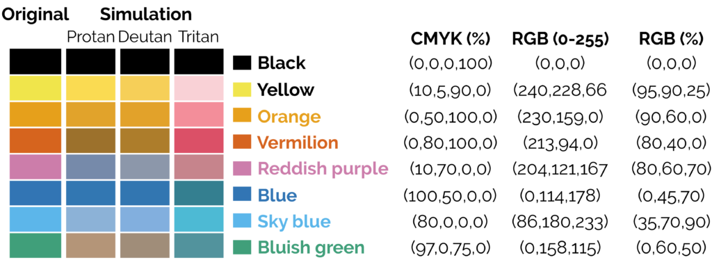
- If using a colour map, avoid the standard rainbow. Other rainbows like viridis colour maps can be downloaded. The brightness varies across the rainbow which leads to visual artefacts that do not exist:

The transition between greens to yellow and red are more prominent than the transitions between greens and blues, making stark boundaries that do not exist. A rainbow with equal brightness solves the problem.
Sisneros et al (2016) Chasing Rainbows: A Color-Theoretic Framework for Improving and Preserving Bad Colormaps. https://doi.org/10.1007/978-3-319-50835-1_36
-
Keeping readability in mind with text size/font and similar considerations
-
“First key point. Brief Answer to questions. (FIXME)”
Data exploration and insights
Let us now create two different DataFrames and perform the merging operations on it.
# import the pandas library
import pandas as pd
left = pd.DataFrame({
         'id':[1,2,3,4,5],
         'Name': ['Alnus', 'Agrostis', 'Betula', 'Vaccinium', 'Dactylis'],
         'subject_id':['sub1','sub2','sub4','sub6','sub5']})
right = pd.DataFrame(
         {'id':[1,2,3,4,5],
         'Name': ['Calune', 'Fallopia', 'Stachys', 'Stellaria', 'tiphy'],
         'subject_id':['sub2','sub4','sub3','sub6','sub5']})
print left
print right
- Data Visualisation as a tool
- Reference: https://helenajambor.wordpress.com/2022/01/04/science-visualization-trends-of-2021/
Statistical analysis
Selection of appropriate statistical method is very important step in analysis of data. A wrong selection of the statistical method not only creates some serious problem during the interpretation of the findings but also affects the conclusion of the study. In statistics, for each specific situation, statistical methods are available to analysis and interpretation of the data. To select the appropriate statistical method, one need to know the assumption and conditions of the statistical methods, so that proper statistical method can be selected for data analysis. Other than knowledge of the statistical methods, another very important aspect is nature and type of the data collected and objective of the study because as per objective, corresponding statistical methods are selected which are suitable on given data. Incorrect statistical methods can be seen in many conditions like use of unpaired t-test on paired data or use of parametric test for the data which does not follow the normal distribution, etc., Two main statistical methods are used in data analysis: descriptive statistics, which summarizes data using indexes such as mean, median, standard deviation and another is inferential statistics, which draws conclusions from data using statistical tests such as student’s t-test, ANOVA test, etc.[
Type and distribution of data used
For the nominal, ordinal, discrete data, we use nonparametric methods while for continuous data, parametric methods as well as nonparametric methods are used. For example, in the regression analysis, when our outcome variable is categorical, logistic regression while for the continuous variable, linear regression model is used (https://www.ncbi.nlm.nih.gov/pmc/articles/PMC6206790/).
The choice of the most appropriate representative measure for continuous variable is dependent on how the values are distributed. If continuous variable follows normal distribution, mean is the representative measure while for non-normal data, median is considered as the most appropriate representative measure of the data set.
Similarly in the categorical data, proportion (percentage) while for the ranking/ordinal data, mean ranks are our representative measure. In the inferential statistics, hypothesis is constructed using these measures and further in the hypothesis testing, these measures are used to compare between/among the groups to calculate significance level.
Case Study:
A Researcher wants to compare the diastolic blood pressure (DBP) between three age groups (years) (<30, 30–50, >50). If the DBP variable is normally distributed, > mean value is the representative measure and null hypothesis stated that mean DBP values of the three age groups are statistically equal. In case of non-normal DBP variable, median value is the representative measure and null hypothesis stated that distribution of the DBP values among three age groups are statistically equal. In above example, one-way ANOVA test is used to compare the means when DBP follows normal distribution while Kruskal–Wallis H tests/median tests are used to compare > the distribution of DBP among three age groups when DBP follows non-normal distribution.
Similarly, suppose he wants to compare the mean arterial pressure (MAP) between treatment and control groups, if the MAP variable follows normal distribution, independent samples t-test while in case follow non-normal distribution, Mann–Whitney U test are used to compare the MAP between the treatment and control groups.
Other Statistical methods
- Logistic regression analysis is used to predict the categorical outcome variable using independent variable(s).
- Survival analysis is used to calculate the survival time/survival probability, comparison of the survival time between groups as well as to identify the predictors of the survival time of the subjects (Cox regression analysis).
- Receiver operating characteristics (ROC) curve is used to calculate area under curve (AUC) and cutoff values for given continuous variable with corresponding diagnostic accuracy using categorical outcome variable.
- Diagnostic accuracy of the test method is calculated as compared with another method (usually as compared with gold standard method).
- Sensitivity (proportion of the detected disease cases from the actual disease cases), specificity (proportion of the detected non-disease subjects from the actual non-disease subjects), overall accuracy (proportion of agreement between test and gold standard methods to correctly detect the disease and non-disease subjects) are the key measures used to assess the diagnostic accuracy of the test method.
- Other measures like false negative rate (1-sensitivity), false-positive rate (1-specificity), likelihood ratio positive (sensitivity/false-positive rate), likelihood ratio negative (false-negative rate/Specificity), positive predictive value (proportion of correctly detected disease cases by the test variable out of total detected disease cases by the itself), and negative predictive value (proportion of correctly detected non-disease subjects by test variable out of total non-disease subjects detected by the itself) are also used to calculate the diagnostic accuracy of the test method.
Summary of these methods can be found here https://www.ncbi.nlm.nih.gov/pmc/articles/PMC6639881/table/T3/?report=objectonly
Communicating Results
- What elements are involved
Producing figures
- Best practices
- Versions
- Publication with persistent identifier
Conclusion
- What gaps have we filled in this section
- Project management overview
Resources for taking this to next level
- https://the-turing-way.netlify.app/collaboration/new-community.html
- Data Visualisation as a tool
- Reference: https://helenajambor.wordpress.com/2022/01/04/science-visualization-trends-of-2021/
Key Points
First key point. Brief Answers to questions. (FIXME)